

2024 has been a great year for new Excel formulas. From enjoying updates to the well-loved VSTACK to better analyzing Pivot tables, discover the most time-saving functions and all the resources you need to master them. Read on to make your work life easier!
Discover the Latest New Excel Formulas and Functions
Insert Pictures into Cells
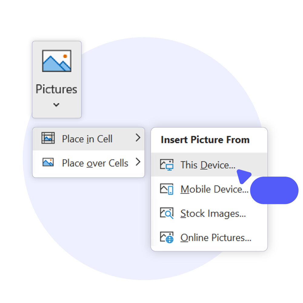
Did you know you can now insert pictures into cells? There are several ways of doing this, but if an image is saved to your PC, the simplest is probably via your Excel ribbon.
Follow these four easy steps:
- Click on the cell you’d like to insert a picture to
- Hover over ‘Place in Cell’ > ‘This Device..’
- Find your picture in File Explorer
- Insert!
Need the picture bigger?
If you want the picture bigger so it overlays multiple cells, simply click on ‘Place over cells’ and it will size up accordingly.

Want to learn more? Discover Microsoft’s guide on inserting pictures into Excel
Split Text into Multiple Rows with TEXTSPLIT
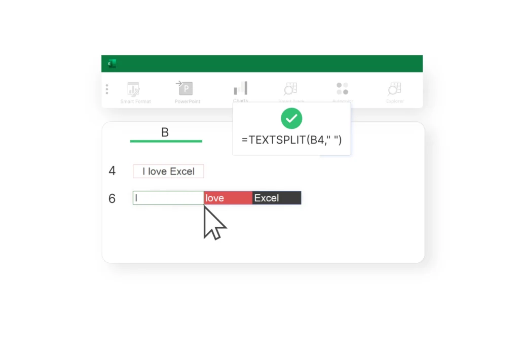
TEXTSPLIT is the inverse of TEXTJOIN. It lets you split text into multiple columns/rows. Like TEXTJOIN, this new Excel feature uses a given delimiter (i.e. space or comma) to separate the text over the desired cells.
Basic TEXTSPLIT Formula
To separate the string in B4 horizontally, enter the following formula into B6:
=TEXTSPLIT(B4, “,”)
In this case, the comma enclosed in double quotes (“,”) is your delimiter.
For more advanced uses of TEXTSPLIT, see the following resources:
Extract Text with TEXTBEFORE and TEXTAFTER
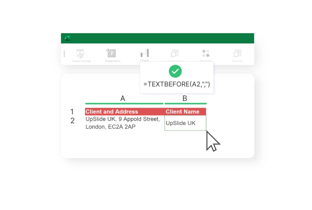
This feature will work wonders if you need to extract text from the beginning or end of a cell.
TEXTBEFORE pulls out all text before a given delimiter, while TEXTAFTER does the same with text after that delimiter.
Extracting the First Word From a String
Enter the following formula:
=TEXTBEFORE(A2,” “,1)
Extracting the First Two Words From a String
Enter the following formula:
=TEXTBEFORE(A2,” “,2)
Extracting the Last Word
Enter the following formula:
=TEXTAFTER(A2,” “,1)
Looking for more advanced uses of these Excel functions? Take a look at TEXTBEFORE and TEXTAFTER to discover more ways of extracting text and boosting your productivity in Excel.
Top Tip
If you regularly work between Excel and PowerPoint, discover our guide on how to link Excel to PowerPoint.
Analyze Portions of Your Data with TAKE and DROP
Take and Drop is a useful new Excel feature that’s great for analyzing a portion of your data. You can keep (TAKE) or remove (DROP) a given number of columns/rows from the start or end of an array.
TAKE: Extract the First Two Rows of Your Data
If you’d like to extract data from the first two rows, just enter the following formula:
=TAKE(A2:B6,2)
TAKE: Extract the First Column of Your Data
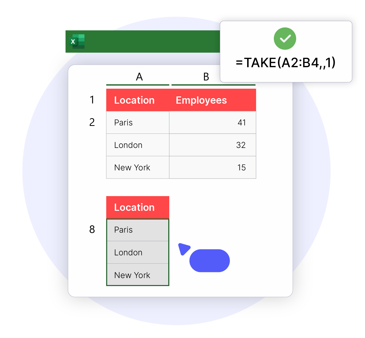
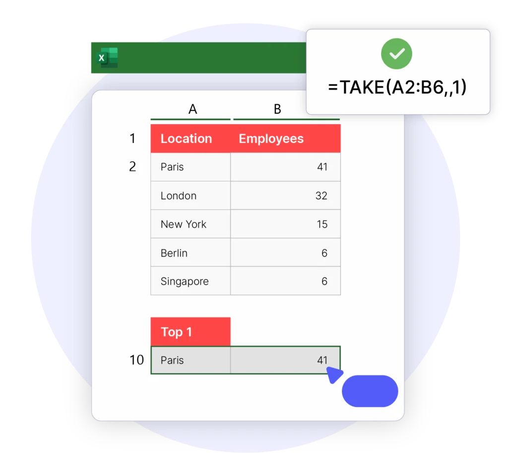
You can also tweak the formula to extract the first column. For this, you’d enter:
=TAKE(A2:B4,,1)
This only scratches the surface, so take a look at Microsoft Support’s guide and master the TAKE function and DROP function in minutes.
Extract Specific Data Sets with CHOOSECOLS and CHOOSEROWS
These brand-new Excel formulas make it easy to extract specific columns (CHOOSECOLS) or rows (CHOOSEROWS) from a range of data sets – whether the data is next to each other or located a few cells away.
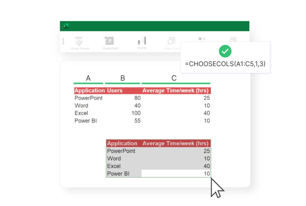
CHOOSECOLS
To extract data from the “Application” and “Average Time” columns, use the following formula:
=CHOOSECOLS(A1:C5,1,3)
For a deeper understanding of these handy new Excel functions, check out Microsoft’s Support guides:
Top Tip
Regularly using Excel as an analyst or associate? Discover our list of the top six Excel financial functions.
Combine Arrays of Data with VSTACK and HSTACK
VSTACK and HSTACK allow you to combine two or more sets of arrays vertically (VSTACK) or horizontally (HSTACK). These new Excel functions work with dynamic arrays and ranges with large source sizes, saving you time.
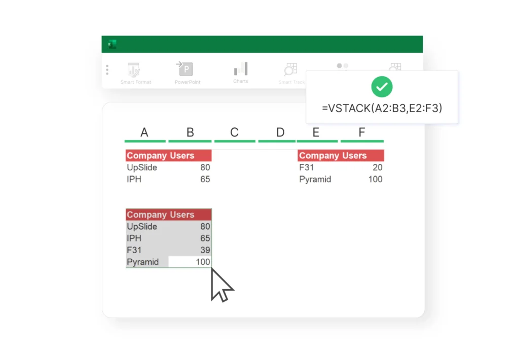
VSTACK
In this example, we’ve combined data from columns A/B and E/F.
To do this, enter the following formula into the cell you’d like to extract all the data to:
=VSTACK(A2:B3,E2:F3)
Voila! Your data from both arrays has now been combined vertically.
For a quick tutorial, these guides from ExtendOffice go into a lot of detail on each new function:
New ‘Show Details’ Button in Pivot Tables
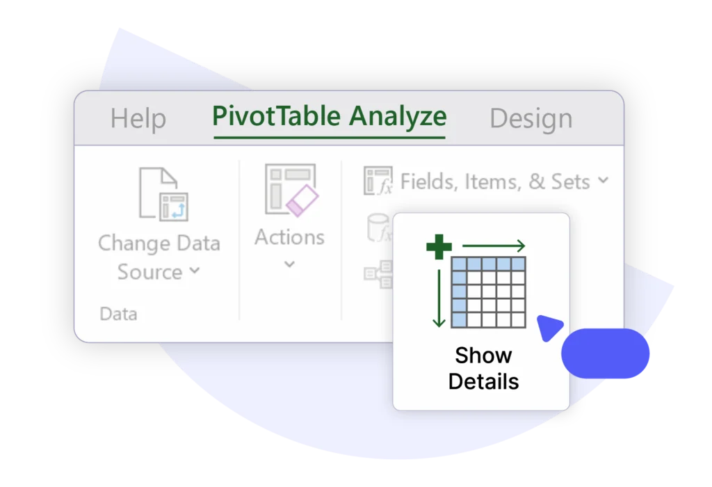
Drill deeper into your Pivot Table data with the brand new ‘Show Details’ button in Excel (it carries out the same function as double-clicking a value cell).
To find this new button, just select your Pivot Table and navigate to ‘Pivot Table Analyze’ in your ribbon.
Once clicked, a new sheet will open to the left with more detailed information, along with a title that states where the data source is from. This is great for simplifying and speeding up your analysis.
BONUS Video Tip: Top Excel formulas in 2024
Prefer a video tutorial? Check out our favorite guide to 2024’s new Excel functions below.
Thanks to Samina Ghori, you can get to grips with these useful new functions in just 15 minutes.
Feeling Confident?
Hopefully, you’re now feeling confident with these handy new Excel formulas and functions. We’ll regularly update this page with new top tips, so please feel free to bookmark it and refer back to it later!
For more efficiency tips and tricks, discover more time-saving Excel resources so you can streamline your workflow and make your work life easier: