When working in finance, Excel is such a powerful tool for manipulating and displaying data to make concise and impactful reports.
With so many shortcuts and formulas it is sometimes easy to breeze past the basics. So here are our basic tips for making the most out of Excel.
Wrap Text
Isn’t it annoying when text in Excel seems to continue horizontally forever across other cells? To solve this, simply go to the Home tab > then to Alignment group and you will be able to wrap it! Or press Alt + Enter, which will allow you to make a new line.
The Status Bar
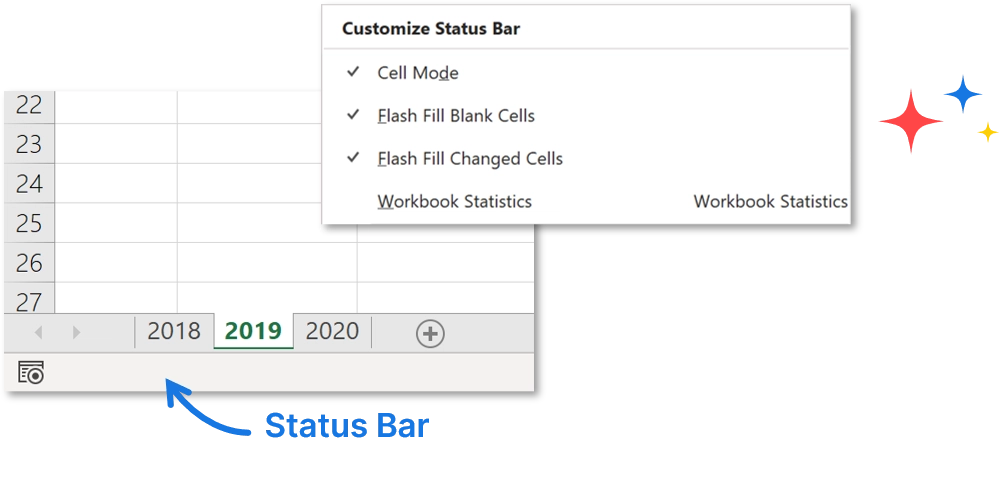
A little-known trick that can provide you with lots more information about your Excel sheets is being able to change the information displayed on the bottom bar of your spreadsheet! All you need to do is right click and select what you would like to be shown!
For instance, here we can choose to add access to our Workbook statistics in just one click:
Diagonal Line in Cells
Diagonal lines across cells are effective to show a no result area so your tables don’t look incomplete. To do this go to Home > Font group > Borders > More Borders and select the Diagonal line!
Flash Fill
This tool analyses data for patterns, in order to be able to automatically fill cells! For example, you have a range of dates from B1:B10 and you want to display the month from those dates in column C. Type the month of the first date in C1, next go to cell C2 and use the shortcut CTRL + E.
Expand the Formula Bar
If you need more space to view your formula, simply hover your cursor along the bottom edge until the vertical, two-headed arrow appears and simply drag the bar up or down to create more (or less) space. Or use the shortcut Ctrl + Shift + U.
You can also indent these formulas just by clicking Alt + Enter, great for making long formulas easy to read.

Enter and Edit a Cell
You can see which mode you are in from the bottom left-hand corner.
Edit mode allows you to edit directly in the cell and will allow you to navigate within the formula using the arrows. But when in this mode, you will not be able to apply conditional formatting or change the alignment of the cell contents.
Ready mode, on the other hand, allows you to navigate normally around the worksheet using the arrows.
Press F2 when on a specific cell and that will allow you to see which cells are being used in the formula.
Highlight Blank Cells
Once a graphic charter has been applied, it is easy to skim past cells which don’t contain a value. To find out if this is the case, select the data you want to check through, go to the Home tab > Editing group > Find & Select > Go To Special and in the dialogue box select ‘Blank’ and click ‘OK’.
You can also highlight the cells you need by selecting other Go To Special options according to your needs!
Conditional Formatting
This is helpful when you want to highlight specific data, but don’t want to manually review the data set – for example if it’s particularly large.
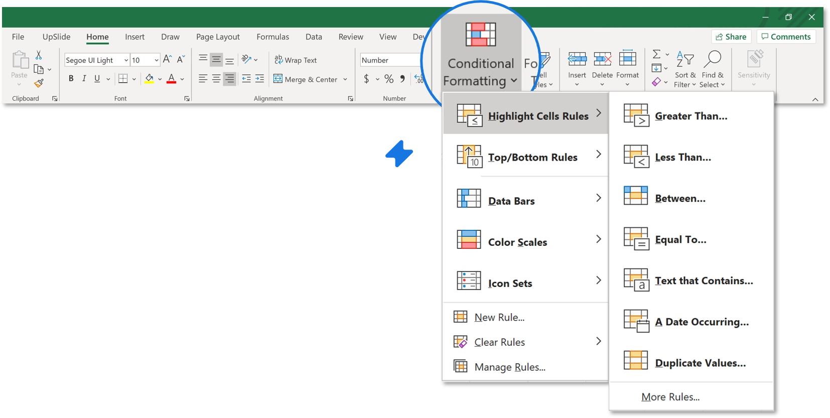
To do this: select your data range, go to the Home tab and in the Styles group go to Conditional Formatting > Highlight Cells Rules > select which rule >and enter your values.
You can also use conditional formatting with a formula which can be used across a range.
Goal Seek
This is a helpful tool which helps you avoid fiddling around and guessing values. If you know the result that you want to get from a formula, use Goal Seek to find the input value that produces this result.
On the Data tab > in the Data Tools group > click What-If Analysis > and then click Goal Seek.
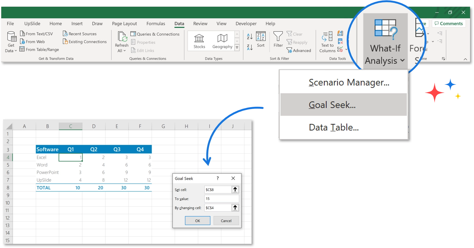
In this example, we used Goal seek to find out how many users we needed in Excel to meet our Q1 target of 10 users.
Freeze Panes
If you want to keep part of your worksheet visible whilst scrolling through other parts, you can do this by freezing the plane. This will save you time as you will be able to easily refer and look back to the column or row you have frozen, as you scroll through the data!
On the View tab > go to Freeze Panes > and select what you want to freeze.
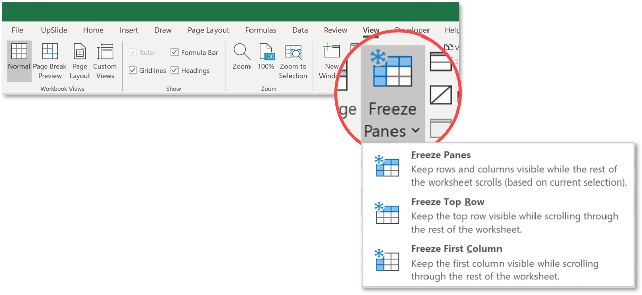
And, you can go one step further. To freeze both a row and a column, select the cell below the rows and to the right of the columns you want to keep visible when you scroll.
Jump to a Particular Cell
When you are deep in an Excel worksheet and want to quickly jump to a particular cell, simply go to the Name Box which is just left of the formula bar > type your cell name in > and press Enter.
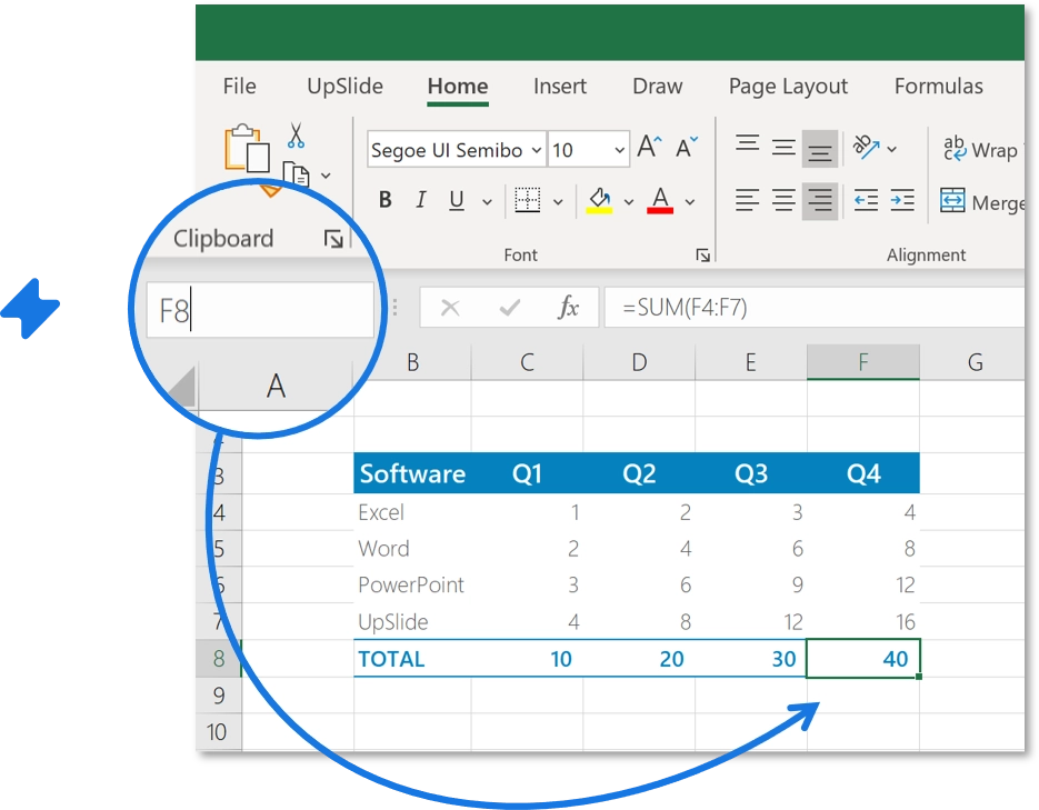
You can also give cells a name to make this even easier. All you need to do is go to Formulas > Define name. This is very useful for people using VBA codes!
Functions Argument Window
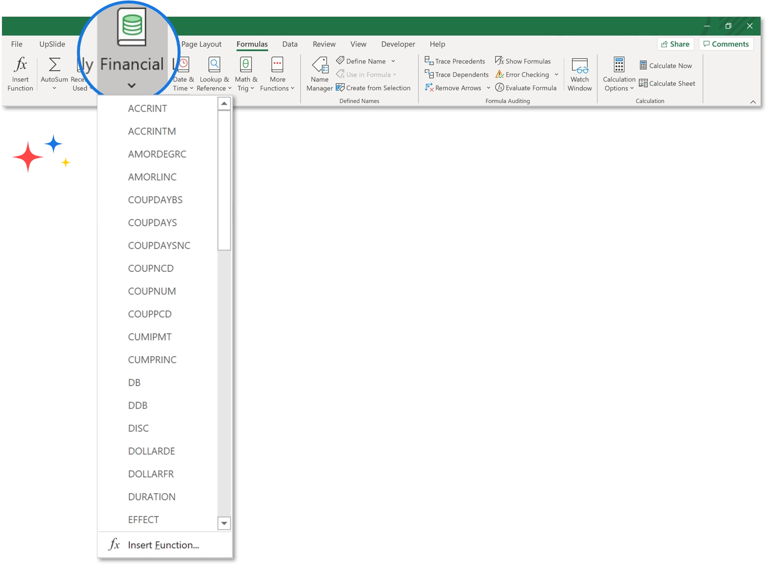
In Excel, under the Formulas tab, there are many premade Excel formulas which can be used with specific values called ‘arguments’.
By pressing Shift + F3, whilst on a cell containing a formula, you will be able to see all the arguments in the function, which is really helpful if you need to see which data is being used in this formula to better understand it. You can also click on Fx at the left side of the formula bar.
Structured References
These are references to a column or table instead of individual cells. So instead of writing =F6-C6 I can write the below:

Not only is this easier to understand but also saves a lot of time if you know what your tables are called. It does require you to adapt the way you usually write your formulas, but once you’re used to it it can save a lot of time.
However, be aware that this only works with tables! You can do it outside of the table by first referencing your table and then the column. It’s convenient as you can make sure to include the whole column and not miss anything out.
Trace when Deleting
This is great when you want to delete a sheet but aren’t sure if there are formulas that are dependent on it. First of all, select a cell that might possibly contain references in a formula on another sheet, then press the Trace Dependents button on the Formulas tab in the ribbon. The keyboard shortcut for Trace Dependents is: (making sure to select the cell first) Alt+T+U+D.

If the Trace Dependents function finds any formulas in other sheets that depend on the selected formula, then a dashed arrow will appear with a spreadsheet icon at the end of it. You can clear the arrows by clicking the “Remove Arrows” button just below.
What’s more, you can do the opposite of this, by clicking on ‘Trace Precedents’, as seen in the image above.
Turn Rows into Columns and Vice Versa
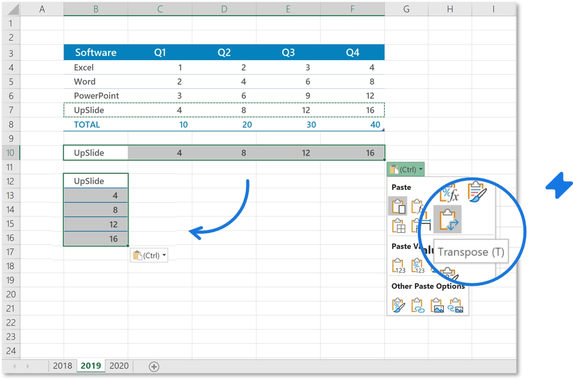
Changing the layout of a table can waste a lot of time. If you want to make a row into column Copy your data > click Paste special > check the Transpose box and click OK to switch the orientation!
Hide Data
Sometimes data is important, but you just don’t want it to be seen on the spreadsheet. The solution to this is selecting what you want to hide by clicking the letter/s (to select the column/s) or numbers (to select the row/s) header, right click and select ‘hide’. You can unhide them by following the same process.
If you just want a hide a few pieces of data, Select the cells > right click > and select Format Cells. On the Number tab > go to Category > select ‘Custom’ and in the type bar enter three semicolons (;;;). You will still be able to use the numbers in formulas but they just won’t be visible!


